We’ve moved all posts over to the eDNA Collaborative site, which seems like a better home for the blog.
Legend of Zeta
By Zack Gold
A key aspect of ecology is trying to compare the communities of species between different sites to answer the seemingly simple question – is this ecosystem different from that other ecosystem over there and how is it different? And a second, much harder but more important question – why?
Sometimes answering to the first question is as trivial as it seems: my two pandemic trips were kayaking through a mangrove with horseshoe crabs and tarpon in the Florida Keys and cruising with salmon and Belugas through a glacially fed river in Turnagain Arm, Alaska. Not a single species overlapped, at least that I could see without a microscope and excluding Homo sapiens. I can say without a single shred of doubt that these ecosystems are different. The second question of why turns out to not be all that hard this time – water temperature and air temp are ~ 25˚C in Marathon Key today compared to a balmy 1˚C and -2.7˚C water and air temperature respectively in Girdwood, Alaska. And undoubtedly the 0.75 m tidal cycle in the Keys vs. 10.6 m tidal cycle in Turnagain Arm as well as the biologically formed white coral derived sand vs. glacially derived silty beaches all play a huge role too. Clearly it is easy to compare ecosystems separated by >8,000 km.

Trumpet fish on Looe Key in Florida
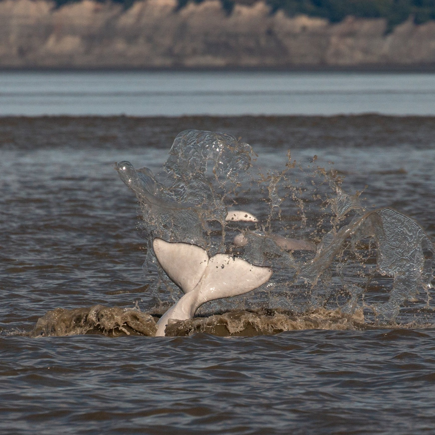
Beluga whale in Cook Inlet, Alaska
But comparing communities far smaller geographic scales, say comparing the reefs out my front porch on Marathon Key to the next reef 5 km down the road, and determining whether or not those are different is a much more arduous undertaking.
The first way you can go about comparing these two reefs is to just count all the species you can find at each site (which again is a heck of a lot harder than it seems, especially in the ocean). In ecology terms– the total number of unique species at a given site is the species richness and is one metric of alpha diversity. We can then compare the total richness from one site to another. Say 20 species at site 1 in front of my porch and 40 at site 2 down the road. This is great, and gives us some information about both reefs, but just counting richness misses a lot of facets of the potential comparisons to be made between each site.
The next-higher-level comparison you can make beyond just the number of species at each site alone, is to compare how many species are shared between these 2 sites – also known as beta diversity. Maybe all 20 of the species at site 1 are also found at site 2. If that’s the case you can definitely make the argument that site 2 is a lot more diverse than site 1 and that site 1 and 2 have decent species overlap – at least a lot more overlap than Alaska and Florida. For much of the comparisons in ecology this is where our comparisons end. You probably do a more thorough surveying with 30 reefs, but most folks still just compared each pairwise combination of sites (site 1 vs. site 2, site 1 vs. site 3, site 2 vs. site 3, etc.). What if you looked at how many species are shared between 3 sites or 4, or – woah get ready - all 30 sites! In short, sticking to beta diversity seems like you are missing an awful lot of higher-level comparisons that one could make.

This is where the legend of zeta begins – creating a scalable metric to be able to compare multiple communities beyond just pairwise comparisons. An important start to this story is that zeta diversity and frankly a lot of my thinking on comparing biodiversity across different scales comes from reading the incredible work of Professors Melodie McGeoch and Cang Hui. Please check out their papers here, they are a lot better at math than I am and made some really wonderful tools for implementing this. I write this blog post as a gateway into thinking about comparing biodiversity at higher scales and to encourage you to use zeta diversity in your ecological thinking. Part of this is inspired by my own admission that there was a steep learning curve to breaking into the zeta diversity framework from just reading the papers. Hopefully this helps break it down and makes it a little easier to incorporate zeta diversity into your own ecological thinking!
Back to zeta: Clearly, only conducting pairwise comparisons between sites is limiting, especially when you have dozens of sites. This is even more limiting when using eDNA metabarcoding when folks now routinely get hundreds of communities to compare often spanning a range of scales from multiple technical, bottle, station, and site replicates! So how do you go about comparing 30 communities at once?
The story begins by introducing you to the key characters of the legend of zeta. First we encounter the "zeta order". Zeta order is surprisingly not like space cult from the Dune universe, but is actually just the number of communities being used in a specific comparison. For example, a zeta order of 3 can be 3 sites or 3 eDNA samples while a zeta order of 4 could be 4 sites or 4 PCR technical replicates (you get the picture). So when you read a sentence about comparing across zeta orders, the authors are referring to comparisons across different numbers of regions or sites or samples, etc. The unit is entirely dependent on the sampling scheme employed and questions being asked. For example, you could be comparing technical replicates within sites or water bottles within sites or sites across a region. Zeta order is just an abstract term for the number of communities being compared.
Second, you encounter "zeta diversity". Zeta diversity is a key metric of this framework that also has nothing to do with tin hats. Zeta diversity is the number of shared species for a given number of communities (zeta order). In our example of reefs above, there were 20 species shared between sites 1 and 2. So you have a zeta diversity of 20 and a zeta order of 2 (2 sites). But importantly, we can compare zeta diversity at a whole range of zeta orders for as many sites as we have. Thus we can calculate the zeta diversity of 30 sites which is just how many species are shared across 30 sites, essentially just the middle of the 30 circle overlapping venn diagram (do not try this at home). Since you expects fewer species to be found across more and more communities sampled, therefore you would logically expect the zeta diversity to decrease with zeta order. In most ecosystems, there are a few species that are very common and a lot of species that are rare. This decrease in zeta diversity with more communities compared is coined as “zeta decay”[insert space zombie reference]. Importantly, you can compare the rates of zeta decay, say between different eDNA samples taken on coral reefs from different regions in Indonesia, and see if samples taken from different reefs in one region have higher species overlap than the other.
We did exactly this in our recent paper sampling eDNA across Indonesia and found that within the most biodiverse sites within heart of the Coral Triangle there was much steeper zeta decay than within sites in western Indonesia. This is telling us that as you sample more and more sites in the heart of the Coral Triangle, there are fewer and fewer overlapping species shared among the many sites sampled whereas in western Indonesia, there is higher diversity shared across sites. Therefore, the rate and shape of zeta decay is a metric of community turnover across samples or sites. This can also be extended to how zeta diversity declines with distance to see if sites closer to each other share more species than sites further apart. Zeta decay can also be looked at across any other variable (temperature) which makes it a powerful metric.
Third you encounter “species retention rates”. This one is clearly not a character from a SYFY original movie. The idea of species retention rates is to see what fraction of the community is still shared as you keep adding more sites. Species retention rates are calculated using the ratios of zeta diversity at different consecutive zeta orders. This is essentially looking at what fraction of the middle of the Venn diagram is still overlapping as you add an additional site/sample. Say you had 20 species shared between 3 sites, you can ask what fraction of species are still shared when you add a fourth site. What percentage of species in the middle of the 3 circle Venn diagram are still there in the 4 circle Venn diagram. You keep doing this until we run out of zeta orders and you can then compare how species retention rates change with more and more sites compared against each other.
Conceptually, the expected change in species retention rates is a little more complicated than zeta decay, so bear with me. Say you have an ecosystem with a lot of rare species and a few common species across all sites – say all vertebrates that live in large North American cities. As you keep surveying more sites, you would expect the species retention rate to first rapidly increase because we lose all the rare species that are not shared between sites. You then expect the species retention rate to asymptote when you are left with the handful of species found in every site. In the North American cities example, you can more or less find mice, racoons, coyotes, crows, and pigeons in basically every city from Florida to Alaska. As soon as you throw in a Seattle, New York, or LA to the 3 way comparisons of comparing multiple cities then the rare urban species like iguanas in the Florida Keys and Grizzly Bears in Alaska are no longer retained. So you would expect in this scenario that you would rapidly asymptote to the handful of species that have more or less learned to live with us. What’s cool is that you can compare species retention rates between groups. For example, you could calculate the species retention rates across different types of cities and see if you saturate species retention rates faster in urban vs. rural environments.
Importantly though, you do not always observe a nice saturation of species retention rates. For example, what happened in our data from Indonesia. Here, we observed an initial increase in species retention rates (more shared species with more sites sampled) followed by a decline, especially in our two most heavily sampled regions in the heart of the Coral Triangle. With this “bell curve”, you first follow the pattern described above in which rare species are not shared between sites, but then since there are very few species shared between a lot of sites (if any at all), species retention rates decline towards zero. This pattern can arise be because 1) only some of your sites are similar and the rest of your sites are completely different from each other (very high community turnover) or 2) you under sampled your sites so badly that a lot of your sites look completely different from each other just because you missed shared species.
In our Indonesia study, we are quite confident that we observed some combination of the first and the second pattern since many sites even on the same island had nearly no overlapping species and we under sampled nearly every region (according to species rarefaction curves), especially in the heart of Coral Triangle. Part of our horrendous under sampling was due to a shockingly unexpected finding in our eDNA metabarcoding samples of a maximum number ASVs (~100-150) found in 1 L of sea water using MiFish primers. This was true across Indonesia despite there being literally a 2 order of magnitude decline in fish diversity across where we sampled. AND, this was true even for a bottle of water from Southern California which has 200x fewer fish species than Raja Ampat! This was definitely surprising and suggests we under- sampled Indonesia fish diversity by a legendary margin. In other words, we did what everyone else does when they survey reefs in Indonesia because it’s ridiculously difficult to survey for >3K species of fishes in an area not that much bigger than LA county. Thus, in probably a shock to absolutely no one, ~30 L of water from the most biodiverse marine ecosystem on the planet did not get anywhere near saturating diversity.
So if you are going to use eDNA in hyper diverse marine environments you will need to take a TON more samples than you do in low diversity environments like Southern California, or Washington, or Alaska. Our estimates suggest it would require 300 samples in Raja Ampat to reach the same level of saturation as a few dozen samples taken in western Indonesia. Sampling for total fish biodiversity with eDNA is thus probably infeasible unless the technology changes or gets a lot cheaper. Still 300 samples is ~$20k worth of processing and honestly a total bargain compared to what it would cost to do 300 full blown scuba surveys.
In our study, we were able to use the zeta decay and species retention rate metrics to explore community turnover across Indonesia fish diversity. We found almost entirely different fish communities from every reef we sampled within the heart of the Coral Triangle with higher zeta decay and a bell shaped species retention rates. On the flipside we saw that western Indonesia sites had much slower zeta decay and higher species retention rates than almost every other region. Combined with comparing species richness and accumulation curves between regions, we were able to use the zeta diversity framework to recapitulate 150+ years of biogeographical patterns across Indonesia with just a few liters of sea water, all despite under sampling.
Ultimately, the zeta diversity framework allows you to answer the two simple questions – 1) is this ecosystem different from that other ecosystem over there and how is it different? And 2) which species contribute to these differences. It extends our analyses beyond pairwise comparisons to look at the full architecture of community turnover at multiple sampling scales. Hopefully this made thinking about zeta diversity easier and opens the door to going above and beyond with zeta diversity analyses like multi-site generalized dissimilarity modelling which can incorporate multiple environmental variables to identify the drivers of community turnover and help us answer the “why” question.
Where should we sample?
By Keira Monuki
As we continue to use eDNA in marine ecosystems, one large, lingering question remains: where, and how often, should we sample? The ocean is vast, covering most of the globe and spanning across immense spatial scales and almost unfathomable depths. Even relatively tiny areas of interest, such as 1 km x 1 km marine protected areas (MPAs), contain several different habitat types across hundreds of meters of depth. If you sample 1 liter in one corner of an MPA at one depth, is that eDNA sample truly representative of the biodiversity within the entire MPA? While eDNA can improve the scale of monitoring efforts because of its sensitivity (1-3), it is unclear how much of a region’s biodiversity is reflected in one eDNA sample. Therefore, knowledge about the spatial and depth variation of eDNA signatures is crucial to figure out how many bottles of water to take and where we should collect to best maximize biodiversity monitoring efforts.
We set out to fill this gap in knowledge in our recently published study where we collected eDNA samples along a fine-scale depth gradient (0 m at the surface to 10 m at the ocean bottom) in a kelp forest ecosystem (i.e., where you SCUBA dive) to assess how eDNA signatures vary across depth. We also took samples from an adjacent surf zone habitat (i.e., where you surf) to see how eDNA varies across horizontally distinct habitats.

Kelp forest (left) and surf zone (right) habitats. Image of kelp forest illustrated by Emily Hess (https://ucscsciencenotes.com/feature/untangling-kelp-forest/).
We detected 71 species of fish, including many of my favorite marine species like the Shovelnose Guitarfish and California Butterfly Ray. Importantly, we found distinct differences in fish communities across depth. eDNA from surface water communities had fewer total species, and the composition of the communities differed between surface and depth. Most interestingly, this depth variation matched the known ecologies of the fishes: eDNA from pelagic, surface-dwelling species proportionally dominated the surface stations, and eDNA from demersal, bottom-dwelling species proportionally dominated the deep stations. For example, California Grunion and Pacific Anchovy were more abundant at the surface, where they typically like to spend time feeding, whereas Pacific Angel Shark and sanddabs were more abundant at the sea floor, where they like to hang out and bury in the sand.


California Grunion (Leuresthes tenuis) at the ocean surface (left) and Speckled Sanddab (Citharichthys stigmaeus) at the sandy bottom (right). Photos courtesy of Flip Nicklin/Minden Picture and Brian McHugh, respectively.
We also found similar results across horizontally distinct habitats, where species who like to hang out in the surf zone, like the California Corbina and Yellowfin Croaker, were more abundant there, and kelp-dwelling species, like the Kelp Bass and Barred Sand Bass, were more abundant in the samples from the kelp forest. Overall, our results show that eDNA captures ecologically relevant depth and spatial variation of fish species, indicating that eDNA is an accurate snapshot of local marine biodiversity.
Additionally, we found differences in species assemblages across days. The biggest differences were in some of the migratory, highly mobile fishes that swim in and out of nearshore ecosystems, such as Pacific Sardine and Pacific Anchovy. However, it’s important to note that the depth and habitat associations were largely consistent – demersal fishes were more abundant in demersal samples and surf zone fishes were more abundant in surf zone samples across the three sampling days. So, ultimately, the depth and spatial variation we observed was largely consistent over time.
Although our study strongly suggests narrow transport of eDNA in marine ecosystems, there is still a lot to be learned about the fate and transport of eDNA. In particular, we need to reconcile the fact that “fish in bucket” experiments suggest eDNA lasts for days to weeks, while our results from the field suggest eDNA isn’t even transporting across 5 m of depth or 150 m of space. We hypothesize that this is possible if eDNA is constantly being generated, and this recently generated eDNA swamps out the signals of past-generated, degrading eDNA. This is definitely a potentially fascinating line of research going forward.
So, what does this mean for sampling? Well, firstly, it adds to a growing list of evidence that eDNA is a reliable tool to survey hyper-local biodiversity. Our results suggest eDNA is biased towards the species’ whose eDNA was captured within or near that location. On the other hand, this strong depth and spatial variation does mean that samples collected at one location may only reflect the species at that location and may not reflect the biodiversity of other depths or habitats. If you sample in the surf zone, then you are sampling fish immediately within that habitat, not so much the fishes in the kelp forest 150 m offshore. To get a full picture of biodiversity in areas such as MPAs, we would need to sample across depths (at least surface vs. bottom), across habitat types (subtidal kelp forest, sandy bottoms, surf zones, etc.), and across multiple time points, especially if there are big seasonal biodiversity patterns. This increases the scope of sampling needed for eDNA-based assessments – 1 or 3 L of water at knee-depth height is not reflective of the total biodiversity even within a small MPA. However, one advantage of eDNA is that sampling costs are low enough (~$50 a sample) that increased sampling efforts are likely not cost prohibitive. This is especially true compared to the costs of big boats, personnel, and equipment needed for SCUBA surveys. An added bonus is that the cost of sequencing continues to become cheaper over time, which will only make eDNA more affordable in the future.
So, back to our original question, how frequently and where should we sample with eDNA? The answer, as is the response to basically every question in ecology, is “it depends”. If the goal is to maximize biodiversity with 100 total samples, then you will need to sample multiple depths, multiple habitat types, and across multiple days. If you especially want to capture all the rare species, you should definitely keep on sampling harder. However, if the goal is to compare the dominant rocky reef fish communities inside and outside an MPA, then the most important factor is to be consistent across depth and directly sample the rocky reef, on SCUBA or with a Niskin. Ultimately, our results, and others, suggest eDNA is a snapshot local biodiversity across depth, space, and time.
References:
1. Ely T, Barber PH, Man L, Gold Z. Short-lived detection of an introduced vertebrate eDNA signal in a nearshore rocky reef environment. PLOS ONE. 2021;16: e0245314. pmid:34086697
2. Jeunen G-J, Lamare MD, Knapp M, Spencer HG, Taylor HR, Stat M, et al. Water stratification in the marine biome restricts vertical environmental DNA (eDNA) signal dispersal. Environmental DNA. 2020;2: 99–111.
3. Port JA, O’Donnell JL, Romero‐Maraccini OC, Leary PR, Litvin SY, Nickols KJ, et al. Assessing vertebrate biodiversity in a kelp forest ecosystem using environmental DNA. Molecular Ecology. 2016;25: 527–541. pmid:26586544
Signal, Noise, and Amplicons
By Ryan Kelly, with thanks to Ole, Ezza, Eily, Alex, Zack, Joe, and Helen
Any study has to be concerned with the signal-to-noise ratio, even if we often don’t explicitly measure it. For any phenomenon we want to measure, we accordingly must ask of our measurements: how much of what I’m seeing is driven by randomness? How much is real, non-random signal that reflects the thing I’m trying to measure?
eDNA amplicons are a fairly noisy kind of data. We know this because we sequence individual PCR replicates; the same environmental sample, amplified and sequenced in triplicate, yields somewhat different reflections of the biological community under study. Because these observations arise from literally the same environmental sample, we know the variation among them is noise, rather than signal. This noise is the observation variance due to the combination of PCR and sequencing. If there were no such variance, our replicates would all look identical. [Note: because thinking about multivariate data can make your brain hurt, here we’re treating observations of each taxon as if they are independent of the others, but that’s not really true… the data are compositional, because of finite read-depth. More on this in the future.]
We can express this variance in terms of the difference in communities –- e.g. Bray-Curtis or other ecological (dis)similarity metrics –- or by changes in the number of species detected, etc., or else by looking at the variation in the abundance of individual sequence variants.
In terms of the difference between observations of whole communities (all observed taxa; Bray-Curtis or other), we consistently see dissimilarities of 0.25-0.4 among technical replicates in our datasets. So, on average, we would need to see changes in Bray-Curtis values larger than this between different environmental samples in order to confidently detect any true signal of community change.
At the level of individual sequence-variants (ASVs; or OTUs, or taxa, or whatever your individual unit of study), we can dig into the analysis a bit more deeply. If we treat sequence reads as being distributed according to a negative binomial distribution for a given ASV i, the probability of seeing a given number of reads nReads_i is
nReads_i∼NegativeBinomial(μ_i,ϕ)
And we know replicates from the same sample have a common μ_i, because they are repeated estimates of that same shared phenomenon in the world. The variability in our observations of the world due to the vagaries of PCR and sequencing, then, is captured by ϕ.
If we know ϕ, we can rationally distinguish signal from noise at the level of individual ASVs, estimating which ASVs contain enough signal that we can confidently use them to measure change in the world, and conversely, which ASVs are unreliable indicators of that change (i.e., noise). (Richness is a separate question… ϕ may change the likelihood of detecting a given ASV/taxon, but it does not speak to the likelihood of an observed ASV being a true or false detection). Moreover, if we know ϕ, there’s an argument to be made that we don’t have to sequence individual replicate reactions, saving time and money and sanity.
An Example
Suppose we observe sequence reads from a beaver (Castor canadensis) in a set of three replicate reactions stemming from a common environmental sample in Creek A. Our read-counts in these triplicates are 132, 47, and 90, respectively. At Creek B, we observe beaver read-counts of 52, 73, and 14. (Assume, for simplicity, that read-depth across all replicates is identical; in reality we can account for variable read-depth using another parameter in the model). Fitting probability distributions to these observations lets us ask questions such as: are we confident that Creek A has a greater signal of beaver than Creek B does, given the observation variation?
To start, let’s fit those distributions and plot the results:

These curves capture the variability in our observations at each creek, and they suggest that Creek A indeed has an expected value greater than Creek B (fitted ML values of μ: 89.67 vs. 46.33). But this doesn’t take into account the variability around those means… that is, our noise (ϕ ; fitted values of ϕ are 6.51 and 2.75, respectively).
We can sample from the fitted probability distributions to get a quick estimate of the difference between them:

And the estimated probability that Creek A has a truly greater number of beaver reads than Creek B, after accounting for our observation variance, is 0.839; the estimated magnitude of the difference between the two sites is 43 reads, with 95% CI of -46, 137 reads.
Variance and the Mean
A corollary here is: we can’t say anything about a difference of a few reads here or there; this is probably more noise than signal To go a bit deeper, we’d like to understand how that noise (observation variance) changes as a function of our mean number of reads μ. For example, do we have more confidence in observations with high numbers of reads than we do in observations with low numbers of reads? Should we?
In the negative binomial distribution (or at least, the version we’re using), the variance is μ+μ2ϕ such that as ϕ gets small, the variance goes to infinity… any number of observations becomes not-too-improbable, and therefore our estimated mean, μ, doesn’t have much predictive value. As ϕ gets large, the distribution becomes more tightly concentrated around the mean.
So: large ϕ means less noise.
Because it’s more intuitive to think about than the variance, let’s look at the standard deviation (SD) and the coefficient of variation (CV), which is just the standard deviation divided by the mean. The CV is useful because it immediately gives a sense of signal::noise… where the standard deviation is greater than the mean, CV >1.
As read-counts rise, what happens to the SD? It depends upon the value of ϕ.

(dashed line in the plot shows 1:1 line)
When ϕ = 1, the SD ≈ the mean (until the mean gets close to zero), and so the CV is constant at 1. No matter how many reads you expect (no matter how big your mean is), the standard deviation keeps pace. When ϕ < 1, the SD > mean, and so there is a ton of scatter around our observations, and so it is more difficult to tell signal from noise. As the mean climbs, the SD climbs faster.
When ϕ > 1 and particularly as read-counts start to climb into the hundreds, the SD becomes much less than the mean, and we accordingly have higher confidence that our read-counts are telling us something. The signal is much greater than the noise. If the CV = 0.5 (ϕ=1.33), for example, a mean of 4 reads would have a SD of 2 (the 25th and 75th quantiles would be 1 and 6); a mean of 400 reads would have a SD of 200 (25th/75th = 148, 551). The chance of observing 0 reads when μ=4,ϕ=1.33 is 0.158; the chance of observing 0 reads when μ=400,ϕ=1.33 is 0.001.
And that’s why we have more confidence in the signal when we have large counts of reads… but for this intuition to be really solid, we have to know about our observation variance, captured by ϕ.
Returning to Our Example
Now that we have a better sense of what the variance term ϕ does, what would happen in our worked example of beaver DNA if we had a noisier set of observations (i.e., our ϕ were lower, like 0.5), but we had the same observed numbers of reads?

Leaving aside the obvious issue here that the observed data don’t match the fitted distributions well anymore – which is unsurprising, since we just invented a variance term for this example, with no regard to the observed data – another thing becomes clear: when variance is high enough, the means don’t matter. We would never be able to tell these sites apart with a ϕ = 0.5 and the set of observed values that we have.
And what would happen if ϕ = 30, and our observations were the same as before?

Again, our observations haven’t changed, but their variance has, so it becomes far easier to distinguish one creek’s signal from another’s… our 95% CI on the difference between observations from these distributions is now (2, 89).
The Good News, Perhaps
Of course we would like to drop a level of replication in eDNA sampling, to save time and money and sanity, as I said before. But I hope I’ve demonstrated the value of (technical) replication here… it lets us easily distinguish signal from noise, or tell us when we can’t trust our observations as well as we’d like to.
There are a couple of bits of good news, I think.
First, it seems likely that the variance term, ϕ, is at least reasonably consistent for a given primer set and study design. So we probably don’t have to run every sample in triplicate, but running some samples in triplicate gives us a good sense of the variance across our whole dataset.
Second, because the variance is related to the mean, deeper sequencing depths will mean that more ASVs will be more reliable signals… that is, by increasing your sampling effort, you increase your ability to distinguish signal from noise. Which we probably knew already, but it’s worth celebrating the idea that we can decide whether or not we care about rare things in our data. If we really care about those rare things, we can make them less rare (and more reliable) by sequencing more deeply.
On Rare Reads
By Ryan Kelly
A recent Twitter thread got me thinking more about rare reads in metabarcoding studies. I have, at points in the past, claimed that 1 read is just as valid as 10,000 reads… but under what circumstances (if any) is this true?
The answer will depend upon the purpose of the analysis, but it’s first worth thinking about where reads come from.
Where Reads Come From
Read abundance is itself an artifact of the processes of extraction and PCR and sequencing, probably to a much greater extent than it is a result of biology. For a given taxon/ASV/OTU, there are many ways (process-wise) to arrive at 1 or 5 or 10 reads: perhaps they arise from a truly rare taxon (low biological abundance), or result from a high-abundance taxon that is poorly amplified by the primer set (i.e., low amplification rate, relative to the others in the sample). Perhaps it’s by chance, where variability in the extraction/PCR/sequencing process resulted in an improbably low number of reads for that taxon/ASV/OTU in that particular sequencing reaction, or it could be due to low read-depth of the sample (although I’d usually assume people think about this first). And so forth. The point is: raw read abundance means very little on its own. And therefore, low read abundance means little on its own.
Stochasticity
Insofar as reads are the result of a long chain of analytical steps, each of these steps is subject to a great deal of sampling variation. So raw read-abundance is a random variable, the stochastic outcome of these complex observation processes. Sequence the exact same DNA extract 10 times, and you’ll get 10 different abundances for a given sequence variant. These won’t be 10 *totally* different abundances — I hope — but they will vary enough that we should not expect any one realization of a sequenced sample to be “truth”. Rather, it is one random draw from a very large number of likely outcomes.
This applies with particular force to rare reads, which will — by definition, because of their rarity — only occur stochastically in samples, due to sampling variance. For example: if we estimate that a PCR reaction results in something like 10^13 amplicons, but then we only get 10^7 amplicons out of the sequencer, that means only one in a million amplicons got turned into a sequenced read. This is a massively small sample, and most rare things won’t be sampled; most rare ASVs won’t occur in the sequencing data. If you sequenced the same DNA extraction again in a technical replicate, all of the same *common* amplicons would show up in the replicate, but many of the *rare* amplicons wouldn’t, and instead you would see different rare amplicons… due solely to chance.
So, as a baseline matter, we should see rare things as more obviously stochastic than common things.
Rare Reads and Richness
Because we know that read abundance doesn’t scale predictably with biomass, we often treat metabarcoding data as somewhat-glorified presence/absence data: we turn detections into 1s and 0s, deciding that a taxon (or ASV/OTU) is either detected or it is not detected. Often the first subsequent analytical stop here is an estimate of richness: how many unique entities did I detect in my samples?
Even putting aside the fact that rare ASVs are likely to be stochastic — and so any given sequenced sample surely didn’t approach the total richness present — here we run headlong into another difficult problem: most metabarcoding ASVs are rare, and so rare ASVs contain most of the richness information. But PCR error is also a real thing (see below) and we want to make sure we are only including real biological sequences in our analysis, excluding artifacts of the PCR process. One common way to handle this is to simply throw out all rare ASVs, but (1) this is likely to grossly mischaracterize the true richness in the dataset, given that most (real) ASVs are likely to be rare, and (2) it’s not obvious how to pick a threshold of rarity for separating the wheat from the chaff.
We’ve tried occupancy modeling to help with this in the past — sequencing replicate PCR reactions is useful in identifying real from spurious reads (see here and here, e.g.) — but where a given ASV occurs only once in the entire dataset (or across multiple datasets), one might have to rely on clustering or other distance- or tree-based techniques to identify likely artifacts. For coding genes like COI, looking at the amino-acid translation can help identify artifacts and pseudogenes as well. But there’s no real magic wand as far as I’m aware. The point is to have some analytical reasoning behind the decisions you make here; show your work, and know why you are doing what you are doing.
Rare Reads and Community Ecology
Other analyses don’t treat metabarcoding data as presence/absence, but rather as an assay of community composition. The subsequent analysis is then often Bray-Curtis dissimilarity or something equivalent, asking how different any two samples are from one another. Assuming that metabarcoding data have been appropriately transformed in some way, I think this is probably a statistically acceptable thing to do, even knowing that read abundance doesn’t equate to species abundance; we aren’t asking how different the two realities of our sample communities are, but rather how different the results of our assays of the two communities are.
Here, rare reads mean something a bit different. They tend to get down-weighted by Bray-Curtis and other dissimilarity/distance metrics, in the sense that these metrics are more influenced by high-abundance ASVs than low-abundance ones. But of course, if you’ve transformed the data (see here and here) such that every ASV occurs on a 0-1 scale (or done some similar transformation), all ASVs will be weighted equally in the dissimilarity calculation. And because most ASVs are rare, this will mean rare ASVs have a disproportionately large influence on the analytical outcome.
One way of handling these issues is to collapse into annotated taxa before undertaking community-level analysis. After all, we often care about the community of taxa, rather than the (larger) community of unique sequence variants. But again, there’s no magic wand, and the best that one can hope for is transparent reasoning in handling difficult issues.
Rare Reads and Absolute Abundance
Finally, if one is trying to estimate actual biological abundances from sequencing reads, we have to assess rare reads yet again. This analysis treats read abundance as a result of a set of biological and analytical processes to be modeled, and finds the most likely biological abundance, given the observed reads and some fitted model parameters. Given the amount of variance at each of these steps in the analytical process leading to sequence data, rare reads simply provide very little information to the model. Again, there are many ways to arrive at 1 or 5 or 10 reads, and here the model has no way of figuring out which of these ways is most likely. For example, if we assume observed read abundance for a given taxon is (for simplicity) a Poisson process, with the expected value being (proportional_amplifiable_DNA)*(1 + amplification_efficiency)^N_PCR_cycles, there are lots of places for variability to arise in terms of both process variance (uncertainty in proportional_amplifiable_DNA) and observation variance (uncertainty in amplification_efficiency and the sampling variability of the Poisson process… and this actually is far less sampling variability than we normally see among technical replicates). With large read-abundances, it’s easy to fit this model. With small read-abundances, it’s impossible without more information to inform the model terms.
PCR Errors
Apart from all of these analytical techniques and questions, there is the overriding concern that rare reads could be artifacts of PCR: that is, not real sequences that exist in the world, but rather mistakes of the process. There is a large literature on this phenomenon, and in general, we need some way to distinguish real sequences from spurious ones. I mentioned occupancy modeling above, and clustering as well. DADA2 and other common tools do some of this work for you, but at the end of the day, you have to decide why you believe a sequence read is real vs. spurious, and I hope I’ve made the case that rarity alone isn’t a sufficient reason.
So, then, under what circumstances is 1 read just as valid as 10,000? I think most of the time. Any time you don’t have a very definite reason to believe the 1 read is a spurious artifact of the observation process. But the question of rare reads still bears thinking about, because the cumulative influence of rare reads on an analytical outcome can be quite large.
What’s in a Name?
By Zack Gold
eDNA metabarcoding still never ceases to amaze, a single liter of sea water detecting hundreds of species from bread crumbs left behind. But how much do we trust our identifications of the species we have found?
Any researcher who has had the pleasure (read: nightmare) of taking tens to hundreds of millions (to now billions) of ACTGs and converting them to sequence counts of individual fish species knows that this is not an easy undertaking. And in the multilayered process of quality- control, dereplicating sequences, and assigning taxonomy there are numerous parameters that can be changed along the way (The Anacapa Toolkit has >150). And like tuning the shifters on a bicycle derailleur, changing one parameter can either cause very little change or produce dramatically different results. So besides trying every possible permutation of every parameter (which is impossible, as a practical matter) what do we do to actually test and parametrize the accuracy of our eDNA metabarcoding assignments?
Our recent paper in the California Current Large Marine Ecosystem lays the groundwork for identifying important best practices to trust species assignments. We highlight 4 best practices:
1) Barcoding your species of interest makes a world of difference
2) Curated, regional reference databases outperform global/comprehensive ones
3) Confidence – Resolution Tradeoffs Abound
4) Benchmarking your marker of interest is key: one size does not fit all
First, good high-quality reference databases are critical. You can’t even ask a single question of ecological relevance if you can’t ID a species. With our current methods we can only ID (to species level) what we have barcoded from tissues in hand – and even then, a given locus might not distinguish species from one another (like my nemesis Rockfishes). Even for extremely well studied species like fishes in California, we found that barely 40% had previously been barcoded for the MiFish Universal 12S region. A rough estimate for invertebrates in Southern California from Dean Pentcheff at the Natural History Museum of Los Angeles County is less than 30% for CO1 (so good luck doing a comprehensive benthic invert survey when 70% of species can’t be ID’d right off the bat!).
So why did eDNA work to begin with? Well there was likely a pretty solid match to sister taxa, maybe in the same family or in the same genus, but nothing great. For example, we found >17% of our millions of reads getting assigned to the family Serranidae from kelp forests in Southern California. Nice to know we have a grouper of some sort around, but not that informative especially given there are dozen species this could be matching to, some of which are threatened species and others of which are not. Knowing whether or not it’s the threatened or common species is undoubtedly important to resource managers. However, once we barcoded 605 fish species, then suddenly – BAM! We got species level ID to Kelp bass, arguably the most abundant fish in Southern California rocky reefs and one of the main recreational fisheries targets.

Figure 1. Why adding barcodes helps. In this hypothetical example we can only assign genus level resolution to our eDNA sequence as there are two decently matching barcode sequences on GenBank. However, after adding additional reference barcodes, including our species of interest in orange, we are able to assign species level identification.
So clearly, making reference barcodes works. Putting in the leg work to generate high quality reference sequences pays dividends for eDNA data! (And Pro Tip - make friends with taxonomists and keep them happy since they are the true eDNA heroes). Fortunately, new methods of mitogenome skimming are now cheaper than Sanger sequencing a single gene and cover all potential regions of interest. Barcoding isn’t exactly the sexiest science, but many resource managers would argue that it makes a big difference. Being able to say “hey we found this endangered Giant Black Sea Bass in your marine protected area” vs. saying “we definitely found fish in the ocean” is the difference between decision-relevant science and getting laughed out of the room. So spend the time and effort to barcode your key target species and thank me later.
Second, curated, region-specific databases outperform global, comprehensive ones. On first hand this finding is not necessarily intuitive. You would think having all the data on hand to assign taxonomy would be the best practice, or at least I did. More data = better decisions, right? Nope!
The issue is when you have sister taxa that are not native to your region of interest. In our case this was best exemplified by the croakers. Turns out there are 6 main clades of croakers (family Sciaenidae) in Southern California (Lo et al. 2015), each of which have sister taxa across the Pacific. When you use the global comprehensive reference database (every sequence on GenBank we could get our hands on with CRUX) with species across the Pacific, you can’t get species- or even genus-level resolution of the croakers because each of these 6 clades share nearly identical 12S genes between taxa. However, by only focusing on species that we know to live in the California Current and excluding all the sister taxa from Japan and Panama that we would not realistically expect to show up in our samples, we then have the resolution to differentiate the different croakers native to California.

Figure 2. Phylogenetic Tree of Southern California Croakers (Family Sciaenidae). Species in blue are native to the California Current. Only Seriphus politus, Roncador stearnsii, and Genyonemus lineatus can be distinguished using the comprehensive database. However, excluding non-native sister taxa allows for the identification of the other croaker species native to the California Current. White sea bass (Atractoscion nobilis) is the one species of management concern we were unable to barcode (single tear***).
This narrower focus of course comes with drawbacks, particularly if you are concerned that one of these species is invasive or might migrate to the California Current because of climate change. But on the whole, using a curated reference database will provide the best taxonomic resolution for most applications. Obviously if you suspect an invasive species might be present then include it in your curated database. For now to triple check this, we have been assigning taxonomy to our query sequences twice, once with the regional database and again with the global database to see which sequences are being assigned differently. So far the only differences we have found have been birds and mammals… that is, species present in the global database but not in our fish specific regional database. This could of course be overcome by simply adding in all the barcodes for the marine mammals and birds in the California Current. Curating your reference library also means making sure it includes all the taxa that you expect to be getting!
Third, these findings highlight tradeoffs inherent in eDNA. On the one hand a regional database may increase accuracy for some species, but that decision has the potential unintended consequence of not allowing you to ID an invasive species that you didn’t know was in your eDNA sample. Metabarcoding is littered with these tradeoffs at every step of the process from primer selection to number of technical/sampling replicates to sequencing depth to taxonomic assignment. And often they all boil down to confidence vs. resolution in our data or in statistics – a bias-variance tradeoff.
Here we found that across taxonomic cutoff scores (we use a Bayesian lowest common ancestor classifier, and this is vaguely analogous to percent identity used by other classifiers) there is a tradeoff between accuracy of assignments and the rates of misassignments to the wrong species. This essentially raises the question – which error is worse? Is it worse to under-classify a species (e.g. be super confident but conservative in your Family level assignment when you could have arguably made the genus/species level ID with decent confidence) or is it worse to mis-classify (e.g. assign it to the wrong species when you should have kicked it back to Genus level)?
The answer – the one you probably that don’t want to hear – is “it depends” (of course). If the detection is for an endangered or invasive species and there are potentially millions of dollars of active management on the line triggered by this detection, you better damn well be confident in those detections. You do not want to be the person that misclassifies the pathogen from metabarcoding, drops $$$ to design a new drug/vaccine to target the pathogen, only to find out that whoops we misclassified that barcode and turns out it’s this other species causing the disease... (don’t be that person).
On the other hand, if the goal is to look at the ecosystem level and see how the whole community is changing in response to an environmental stressor, then you can totally afford to make some misclassification calls while increasing your overall accuracy. You might just find patterns that are only visible at the species level, but not at the family level (e.g. Rockfishes are ecologically so divergent from each other but genetically they are almost identical). And you can always cherry-pick a few species to triple check the assignment accuracy via blasting/Sanger sequencing if there are novel findings that pop out because of this. But there is no way that we can hand curate each ASV assignment; nobody’s got time for that. Still, being overall more accurate is arguably often the right strategy.
All of this came from testing just one of the 150 parameters in the Anacapa Toolkit... We can probably ignore a good 100 off the bat since they are probably minor (e.g. cutadapt trimming length), but others like Q scores apparently can make a huge difference (don’t have anything published on this, but we found that Q35 removed ~10 million reads compared to Q30 and led to dramatically increased variability across technical replicates). Clearly, it’s still the wild west out there in terms of parameters and everyone has their favorites either because they were handed down like the thermocycler profile that randomly works and you will never change or because that Tuesday morning after your fifth coffee the day before orals you said 30 sounds like a great number and never looked back. Either way, neither of these methods for conducting science is recommended. Though I truly sympathize in my soul why you don’t want to go back and question your life/PCR/parameter choices.
Which leads us to the ultimate lesson, if we have learned anything from this endeavor of trying to take DNA out of literally thin air/water is that one size does not fit all. You have to test your parameters to know what is going on under the hood in the bioinformatics pipelines. For example, the optimal taxonomic cutoff score, one that best balances confidence and resolution, for the MiFish primer (60) but this is different from the 16S V4 primers (80) and WITS primers (40). If you use the same score for bacterial 16S and throw it at fishes you will only be getting Family level assignments and you will have a much less exciting day than the one where you say: “WOAH I found blue whale in this bottle of water off Santa Cruz Island!”. All of this is to say that taking an optimal parameter from one primer set and throwing it to another is not the way we should be conducting metabarcoding. The 97% taxonomic identity comes from an average of differences in mtDNA between vertebrates. It is truly an abstract average number. We know that this is not even true for all vertebrates (Rockfishes, for example). Does it make sense to apply to crustaceans? Who the hell knows?! But if you don’t test it then you don’t know. And if you don’t know then we are just the blind leading the blind down the mine field of rabbit holes that is metabarcoding taxonomic assignment. If I learned anything from the 90s is that this is a bad way to play Mine Sweeper. You might randomly win, but 99.999% of the time you are going to have a bad day.
So where does that leave us?
We need to be benchmarking each primer set and evaluating the optimal parameter selection for each. Yes, it sounds awfully tedious, but it’s clearly warranted by the data and we have the tools do this (and are working on making them even easier to implement – look out for rCRUX). Robert Edgar has a brilliant set of scripts to run taxonomy by cross validation (TAXXI) to determine how changing a single parameter, reference database, or entire pipeline effects taxonomic assignment scores. The tools are out there and it just takes some legwork to find the optimal settings.
It’s worth checking every piece of your bike to know how it works – changing the large gears has a lot more impact than changing a small gear. Likewise changing the angle of the derailleur hanger can have a huge impact on shifting performance while changing the tension in your barrel adjusters is minor. The only way we are going to climb up this hill of eDNA metabarcoding and be able to effectively and accurately assign taxonomy is to know which parameters are large gears, which are small, and which are barrel adjusters. To do this we are going to have to take our pipelines apart and systematically fine tune the parameters to know which ones matter and which ones not so much. Sure you can borrow someone else’s bike and jump on and try to climb to the top, but I promise you the ride is a lot more enjoyable in low gear. That being said, if your barrel adjuster is off for the ride will you even notice? If you get to the top does it even matter? But for the love of your fellow eDNA scientists and humanity as a whole if you do find the low gear, please, tell your friends. Scream it from the top of mount eDNA. We will buy you multiple cases of beer for saving us from the long arduous slog of parsing sequences so we can get to the “Woah I found Great White Shark off of Palos Verdes” moments a lot faster.
But where did the eDNA in my water sample come from? Thoughts on eDNA transport
By Eily Allan
One of the first questions asked when presenting eDNA data is: “It is great that you found eDNA from beaver in your water sample, but where was the actual beaver?” Unfortunately, the answer is usually unsatisfying as it is either extremely simplified (and therefore probably not quite right and should be taken with a big grain of salt) or extremely complicated…
The problem with this question is that answering it requires considering every other eDNA process to answer it, many of which we still don’t know much about. We need to know 1) how much eDNA an animal sheds (which can vary several orders of magnitude, even within the same individual), 2) at what rate the eDNA is decaying (which can vary with lots of biotic and abiotic factors like temperature - which can also change drastically in a given environment like night versus day or different depths in the water column), 3) what form the eDNA is in and how that will impact its physical transport (think a single cell versus a fecal pellet), and 4) the decisions we make in the lab (more on this later). Harrison et al. 2019 summarizes these processes and their interactions particularly well.
Of course, there is a spectrum of complexity with perhaps a stagnant pond on one end and a deep, dynamic oceanic environment on the other. And regardless of the physical environment, it would be great if we knew that the thing we were studying was stationary, but more likely we have an animal swimming around and shedding eDNA at different points in space and time (and at different rates!).
Ok, so it can get overwhelming quickly. But we can try to isolate things and determine what we can maybe ignore and what we definitely can’t ignore. After eDNA is shed from an animal, theoretically, it can move in the water column by advection (“going with the flow”) and dispersion (aka mixing). We traditionally think in the horizontal direction, but there can also be vertical advection and dispersion (although usually much lower values than their horizontal counterparts), and we also need to consider if eDNA is settling. Finally, in shallow or benthic environments, we should consider if previously settled eDNA is resuspended. So eDNA can theoretically move in a lot of ways, but which ones are important?
We can generally use two approaches. One is to model eDNA as we do with other particles like fine particulate organic matter (FPOM), microplastics, fish larvae, or marine snow. This will give us some basic information about what how far we might expect eDNA to travel based on what we know of how water moves (aka use ocean models). But, it requires a lot of assumptions, and some of which we just don’t know yet (see Andruszkiewicz et al. 2019). Our estimates of transport distances given what we know about the timescale of eDNA decay can be on the order of 10s to 100s of kilometers. So, it’s somewhere to start but maybe not the best approach.
Another method is to conduct field sampling in a very specific way to isolate some of the elements of the problem. Going back to our simplest case of a pond, a recent study (Littlefair et al. 2020) looked at how eDNA is vertically distributed in ponds, and how those distributions change as the lake is stratified (or not stratified) by sampling during different seasons. The authors found that when the lake was stratified (discrete layers of different temperatures), the eDNA is also stratified, and thus not moving up and down vertically. And importantly, different fish resided at different depths, with some preferring warmer or colder water, and the eDNA signals matched the fish occupancy as determined by acoustic telemetry (sound signals). This implies that the depth at which the eDNA is located is the depth at which the animal is located, which is great! But, the water itself was not mixing in that case. When the lake was well mixed (as indicated by the same temperature throughout the water column), the fish occupied many depths and the eDNA was found to be at many depths. But now we can’t separate the fish moving from the eDNA moving after it has left the fish. So not perfect, but this is important and a good place to start - and we obviously need more data and modeling to explore more complicated scenarios.
Moving to a more dynamic habitat, two different studies have now put cages with fish in rivers and measured how far downstream eDNA can still be detected (and how spread out the signal is across the river as you move downstream). Laporte et al. 2020 put fish cages in a very large river (the St. Lawrence River) and used a hydrodynamic model to simulate eDNA concentrations and compare results to field samples. The authors found that eDNA was transported up to 5 km downstream and that lateral mixing (side to side) was minimal. In a much smaller alpine stream, Thalinger et al. 2020 assessed lateral (side to side) and longitudinal (downstream) eDNA transport over different seasons (and thus, drastically different flow rates). The authors found similar results where eDNA was detected up to 1.3 km downstream (the farthest sampling point) and importantly that on small spatial scales (within the first 20 m downstream of the cages), eDNA lateral distribution mostly matched the location of the cages, indicating low lateral mixing. These studies are really important for advancing our understanding of how far downstream we can detect eDNA (also see Shogren et al. 2017, Civade et al. 2016, Deiner and Altermatt 2014, and Pont et al. 2018 for more on transport in rivers).
As far as I know, similar studies in the ocean have not been conducted, but aquaculture facilities could be a good way to sample the “radius” at which eDNA can be detected around a stationary point source. However, in the literature, there are several studies that have found that fish communities determined by eDNA vary on very small spatial scales (Port et al. 2015, Kelly et al. 2018, etc.)? Those imply that eDNA actually can’t move that far from the animal after it has been shed. How can we reconcile the different estimates of how far eDNA can move with these studies? We have been thinking about this a lot and have to continue reminding ourselves of what we are trying to measure and how we are measuring it. Or in other words, it depends on your perspective (and methods).
Basically, there are two ways to ask the question about eDNA transport:
1) How far does a single eDNA particle move?
2) At what spatial scale can you detect differences in communities by eDNA?
Conveniently, these correspond well with the two different ways we currently use molecular tools to find eDNA in water. It makes more sense to answer question 1 with qPCR for just a single species at a time. Question 2, however, requires looking at many species at once and implies the use of eDNA metabarcoding. But eDNA metabarcoding does not do a great job at giving quantitative results for a given species (for many of the reasons Ryan described in a previous blog post – namely, PCR bias and other errors introduced in laboratory processing). And we have to be particularly careful about false negatives in metabarcoding data. If something is not detected via metabarcoding, it might not mean that the DNA (and thus the animal) wasn’t there. Going back to reconciling the long transport distances but small scale spatial differences, we have to remember that they have primarily been answering two separate questions using two different tools (a notable exception is Civade et al. 2016, which looked at eDNA transport using metabarcoding rather than qPCR). So, there is a world in which coho salmon eDNA can be transported 100s of meters but we can still determine that Site A is different than Site B which is only 20 m away because we found coho salmon at both sites, but other fish and invertebrates and diatoms unique to each site.
So… how does this apply to field samples where we found beaver eDNA? First we need to ask how was the beaver identified – using qPCR or metabarcoding? And then we probably need to think about the other processes I mentioned before as it relates to beavers and the water we sampled – like how much eDNA does a beaver shed and how long do we expect eDNA to last in this water temperature? And a final complication to leave you with: what if there were multiple beavers? One might have been 5 m upstream a day before collecting our water sample and another one 75 m upstream and hour before collecting our water sample.
Like I said, it can get complicated! Probably the beaver was less than a kilometer upstream. But who really knows.
How Much is Environmental DNA Information Worth?
By Ryan Kelly
A really practical question for eDNA is: so what? So I can detect all kinds of species in the world with a water/soil/air sample, but what good does that do me, if I already knew these things were there?
The answer, of course, is that there are all kinds of practical reasons that eDNA data might be valuable. An eDNA assay might be more sensitive than other methods of sampling, for example. Or it might be cheaper, more scalable, or more easily automated. But even these advantages might be difficult to sell when existing management programs have been in place for decades — switching methods carries substantial amounts of risk, and there are often institutional barriers to doing so.
So then the next question might be: what information does eDNA give me, relative to what I’m already collecting, and how much marginal benefit does that new information have?
And the answer to that one suggests use-cases that are — to my knowledge, at least — so far relatively rare in the published literature: data-poor situations. The logic goes as follows: if you already have a lot of information about your study system, adding eDNA doesn’t give you much benefit (about the system… although it might be very valuable in terms of assessing the behavior of your eDNA assay). But where you have little existing information, eDNA data is way, way better than what you had before.
Abby Keller’s recent master’s thesis gives the most concrete example that I know of. She’s getting ready to submit it for publication now, but this blog seemed a good place to highlight it.

The setup: European Green Crab is an invasive species in the United States, and is recently starting to invade Puget Sound, near Seattle. The state Department of Fish and Wildlife and Washington Sea Grant spend a lot of time and money trapping sites at which these crabs may (or may not) be present. Some sites have hundreds of traps set over months; others have few, and of course many potential habitats have no traps at all, because there is limited time and money to dedicate to such sampling. Abby sampled water at 20 of the sites with at least some trapping data, used a green crab qPCR assay to test for its presence, and developed a joint model for qPCR and trap data to look at the relative sensitivity of each of the survey methods.

Given this dataset, she could then ask the question I started with: So what? Where did eDNA provide additional value (relative to the existing traps), and where did it not? She found the molecular dataset was particularly valuable at and beyond the known invasion front, where trapping was less intensive, and thus less background information was available. And of course, finding invasive species at and beyond the invasion front is precisely where you would most want to find the rare individuals as they start to show up.

The value of results from a replicated qPCR assay, as measured by the reduction in uncertainty (delta-CV) in the estimate of number of crabs present at a site. Number of existing traps — and so, the existing amount of information about crabs at a site — given on the x-axis. The information value of eDNA is highest when the number of traps is lowest, which is perhaps intuitive, but is especially important where little existing information is available at/beyond an invasion front (here, purple dots) or other location important for management. (Keller et al., forthcoming).
More generally, this example points out the value of eDNA for data-poor situations worldwide. Once you know how well your assay works, it’s quite likely to be most valuable in places where we have relatively little information in-hand.
One Apple, One Orange
(or, “Why does my metabarcoding dataset look different from my visual surveys/nets/traps/etc?”)
by Ryan Kelly (with thanks to Ole Shelton, Erin D’Agnese, Eily Allan, and Zack Gold)
As eDNA datasets have become more common, a frequent and reasonable step for many applications is to compare some eDNA (mainly metabarcoding, sometimes qPCR or ddPCR) results to those of some other, more traditional sampling method. Examples include nets of all kinds, acoustic signals, microscopy, traps, visual surveys, and so on. All are some flavor of “compare and contrast eDNA results and X”, with the idea that if X is an accepted sampling method in ecology or similar field — and if the eDNA results are similar enough to the results of X — then eDNA methods will simply slot into existing survey methods, statistics, and projects, off-the-shelf technological upgrades for existing methods.
But of course, this rarely works so cleanly. Inevitably, we all end up trying to compare one apple and one orange — eDNA data and some other data, collected on the same day in the same place — and perhaps squinting and standing on one leg to show how, in the right light, they might be correlated. But this is madness. (And it’s madness in which we’ve engaged in ourselves; there’s no shame here).
Perhaps the most fundamental way in which eDNA data are different from traditional methods, as a whole, is that the PCR process is exponential. This leads to really different-looking data resulting from metabarcoding studies, in particular. And — principally amplification bias of primer-template matches — the number of sequenced reads from a given species can bear no relationship to the starting (or proportional) biomass of that species in the sampled environment. So eDNA data might be a complete mismatch to, say, visual surveys, or the reads might be 5 orders of magnitude different from the visual counts. And that’s not because eDNA is wrong or inherently flawed, but because small biases get exponentiated and can dominate the underlying signal. Put differently: “normal” ecological surveys happen on the scale you are interested in; eDNA surveys are different because we never observe the eDNA directly, but only an exponentiated, crazy version of it.
Another way eDNA is different is that those same amplification biases aren’t predictable in the way that visual surveys (or whatever) have predictable biases. Primers designed for mammals might amp most mammals (but not all)… just because no grey whale showed up in your dataset doesn’t mean no grey whale was present in the sample. Which is frustrating. And different from most other sampling methods.
Which brings me back to the comparison that many of us would like to do: one apple, one orange. Completely reasonable, and generally doomed to failure, given that there’s no reason to *expect* metabarcoding results to look like visual surveys or net tows — or culture-counts, in the case of microbiome studies. The processes leading to the two datasets are just really different.
The solution lies in understanding this process, and building that into the expectations for your data. Say we have done 35 PCR cycles in a metabarcoding study with primers amplifying mammals. The number of grey whale reads we expect is
s * (b*(1 + a)^35) * uncertainty,
where `b’ is the proportion of the amplifiable DNA present, `a’ is the amplification efficiency (somewhere between 0 and 1, and not predictable in silico) of the primer-template match, and `s’ is a scaling parameter that tells us what fraction of the amplicons put onto the sequencing run were actually sequenced. If we know grey whale as an a = 0.75, and we observe some number of reads on our sequencing run, we can estimate `b’, the amount of whale present.
But what about that uncertainty (error) term? That captures all of the variability that happens sample-to-sample and replicate-to-replicate. It comes from pipetting error, and random sampling error, and so forth. A dataset with technical replicates makes it possible to parse some of these out into separate terms, but ultimately, this is all noise in your data, obscuring the relationship between the amount of a species and the number of reads that come out of the sequencer.
Crucially, it’s clear that the number of reads recovered for a species *does indeed* have a relationship to how much of that thing there is in the world. It’s just that the relationship isn’t linear. And why would we expect it to be, with an exponent of 35 (or 40, etc) in the process?
So all isn’t lost for our apple and our orange. We *do* expect visual counts and nets, etc., to correlate with the `b’ term in the equation above. And where `a’ is high — that is, the primer set does a good job of amplifying the target species, relative to the others in the pool — we expect that correlation to be quite strong. Where `a’ is low, by contrast, the error term swamps any signal in the data, and the number of reads is uncorrelated to observations from other methods.
A somewhat principled cheat for the equation above is to normalize read counts within a taxon… to create an index of eDNA abundance for that particular taxon. (We did this in Kelly et al. 2019, first controlling for different read-depth across samples, and then scaling those proportions within a taxon to create the eDNA index; see also McLaren et al 2019). The index says “all other elements being equal, changes in reads over time — within a taxon, but not between taxa — will track changes in biomass.” You don’t need to know any of the terms in the equation. This approach assumes that `a’ is constant no matter the biological context — which isn’t precisely true, and also, the relative ranks of the efficiencies of species present matters a lot: what if a new species entered the community that had a huge `a’ and swamped everything out? — and elides over the finite read-depth that creates compositional datasets. But it seems to work pretty well in practice… most especially when a species is amplified well by the primer set in hand. And all of those species at the top of your data matrix — the ones with very high read abundances — are, nearly by definition, amplifying very well. (The terrors of compositional data will surely be a later discussion point).
And that whatever the non-eDNA dataset is that you’re using for comparison? That also has some underlying process leading from biological entity in the world to the data on your screen. We just tend not to think about that. Every way of seeing the world has different biases; every data collection is imperfect. So building in information about those imperfections is also a good idea, in terms of a fair comparison. For example, is it likely your visual survey observed all of the individuals that were really present?
In sum, the straight-up apple-to-orange comparison won’t work well. But that’s not to say the eDNA-to-other-data comparison won’t work well. It just takes a bit more analysis before things line up the way you hope they will. This, in more math-heavy language, is what Shelton et al. 2016 was all about, and I’ve been spending the past five years trying to get that into my head as my default view of the world.
First post
Given the discussion on Twitter, it seemed this would be an OK place to (temporarily?) host a blog for discussion of eDNA.