By Zack Gold
A key aspect of ecology is trying to compare the communities of species between different sites to answer the seemingly simple question – is this ecosystem different from that other ecosystem over there and how is it different? And a second, much harder but more important question – why?
Sometimes answering to the first question is as trivial as it seems: my two pandemic trips were kayaking through a mangrove with horseshoe crabs and tarpon in the Florida Keys and cruising with salmon and Belugas through a glacially fed river in Turnagain Arm, Alaska. Not a single species overlapped, at least that I could see without a microscope and excluding Homo sapiens. I can say without a single shred of doubt that these ecosystems are different. The second question of why turns out to not be all that hard this time – water temperature and air temp are ~ 25˚C in Marathon Key today compared to a balmy 1˚C and -2.7˚C water and air temperature respectively in Girdwood, Alaska. And undoubtedly the 0.75 m tidal cycle in the Keys vs. 10.6 m tidal cycle in Turnagain Arm as well as the biologically formed white coral derived sand vs. glacially derived silty beaches all play a huge role too. Clearly it is easy to compare ecosystems separated by >8,000 km.

Trumpet fish on Looe Key in Florida
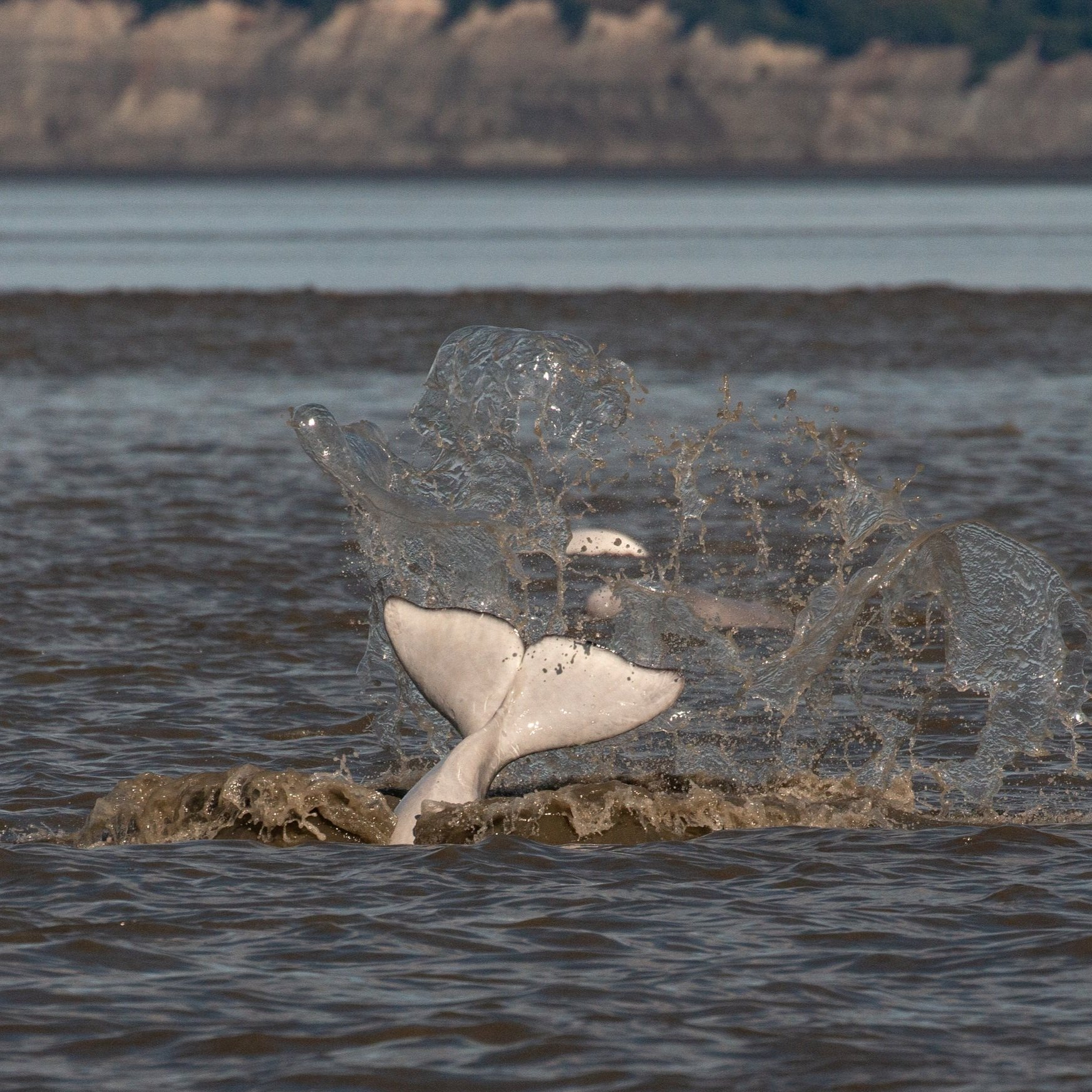
Beluga whale in Cook Inlet, Alaska
But comparing communities far smaller geographic scales, say comparing the reefs out my front porch on Marathon Key to the next reef 5 km down the road, and determining whether or not those are different is a much more arduous undertaking.
The first way you can go about comparing these two reefs is to just count all the species you can find at each site (which again is a heck of a lot harder than it seems, especially in the ocean). In ecology terms– the total number of unique species at a given site is the species richness and is one metric of alpha diversity. We can then compare the total richness from one site to another. Say 20 species at site 1 in front of my porch and 40 at site 2 down the road. This is great, and gives us some information about both reefs, but just counting richness misses a lot of facets of the potential comparisons to be made between each site.
The next-higher-level comparison you can make beyond just the number of species at each site alone, is to compare how many species are shared between these 2 sites – also known as beta diversity. Maybe all 20 of the species at site 1 are also found at site 2. If that’s the case you can definitely make the argument that site 2 is a lot more diverse than site 1 and that site 1 and 2 have decent species overlap – at least a lot more overlap than Alaska and Florida. For much of the comparisons in ecology this is where our comparisons end. You probably do a more thorough surveying with 30 reefs, but most folks still just compared each pairwise combination of sites (site 1 vs. site 2, site 1 vs. site 3, site 2 vs. site 3, etc.). What if you looked at how many species are shared between 3 sites or 4, or – woah get ready - all 30 sites! In short, sticking to beta diversity seems like you are missing an awful lot of higher-level comparisons that one could make.

This is where the legend of zeta begins – creating a scalable metric to be able to compare multiple communities beyond just pairwise comparisons. An important start to this story is that zeta diversity and frankly a lot of my thinking on comparing biodiversity across different scales comes from reading the incredible work of Professors Melodie McGeoch and Cang Hui. Please check out their papers here, they are a lot better at math than I am and made some really wonderful tools for implementing this. I write this blog post as a gateway into thinking about comparing biodiversity at higher scales and to encourage you to use zeta diversity in your ecological thinking. Part of this is inspired by my own admission that there was a steep learning curve to breaking into the zeta diversity framework from just reading the papers. Hopefully this helps break it down and makes it a little easier to incorporate zeta diversity into your own ecological thinking!
Back to zeta: Clearly, only conducting pairwise comparisons between sites is limiting, especially when you have dozens of sites. This is even more limiting when using eDNA metabarcoding when folks now routinely get hundreds of communities to compare often spanning a range of scales from multiple technical, bottle, station, and site replicates! So how do you go about comparing 30 communities at once?
The story begins by introducing you to the key characters of the legend of zeta. First we encounter the "zeta order". Zeta order is surprisingly not like space cult from the Dune universe, but is actually just the number of communities being used in a specific comparison. For example, a zeta order of 3 can be 3 sites or 3 eDNA samples while a zeta order of 4 could be 4 sites or 4 PCR technical replicates (you get the picture). So when you read a sentence about comparing across zeta orders, the authors are referring to comparisons across different numbers of regions or sites or samples, etc. The unit is entirely dependent on the sampling scheme employed and questions being asked. For example, you could be comparing technical replicates within sites or water bottles within sites or sites across a region. Zeta order is just an abstract term for the number of communities being compared.
Second, you encounter "zeta diversity". Zeta diversity is a key metric of this framework that also has nothing to do with tin hats. Zeta diversity is the number of shared species for a given number of communities (zeta order). In our example of reefs above, there were 20 species shared between sites 1 and 2. So you have a zeta diversity of 20 and a zeta order of 2 (2 sites). But importantly, we can compare zeta diversity at a whole range of zeta orders for as many sites as we have. Thus we can calculate the zeta diversity of 30 sites which is just how many species are shared across 30 sites, essentially just the middle of the 30 circle overlapping venn diagram (do not try this at home). Since you expects fewer species to be found across more and more communities sampled, therefore you would logically expect the zeta diversity to decrease with zeta order. In most ecosystems, there are a few species that are very common and a lot of species that are rare. This decrease in zeta diversity with more communities compared is coined as “zeta decay”[insert space zombie reference]. Importantly, you can compare the rates of zeta decay, say between different eDNA samples taken on coral reefs from different regions in Indonesia, and see if samples taken from different reefs in one region have higher species overlap than the other.
We did exactly this in our recent paper sampling eDNA across Indonesia and found that within the most biodiverse sites within heart of the Coral Triangle there was much steeper zeta decay than within sites in western Indonesia. This is telling us that as you sample more and more sites in the heart of the Coral Triangle, there are fewer and fewer overlapping species shared among the many sites sampled whereas in western Indonesia, there is higher diversity shared across sites. Therefore, the rate and shape of zeta decay is a metric of community turnover across samples or sites. This can also be extended to how zeta diversity declines with distance to see if sites closer to each other share more species than sites further apart. Zeta decay can also be looked at across any other variable (temperature) which makes it a powerful metric.
Third you encounter “species retention rates”. This one is clearly not a character from a SYFY original movie. The idea of species retention rates is to see what fraction of the community is still shared as you keep adding more sites. Species retention rates are calculated using the ratios of zeta diversity at different consecutive zeta orders. This is essentially looking at what fraction of the middle of the Venn diagram is still overlapping as you add an additional site/sample. Say you had 20 species shared between 3 sites, you can ask what fraction of species are still shared when you add a fourth site. What percentage of species in the middle of the 3 circle Venn diagram are still there in the 4 circle Venn diagram. You keep doing this until we run out of zeta orders and you can then compare how species retention rates change with more and more sites compared against each other.
Conceptually, the expected change in species retention rates is a little more complicated than zeta decay, so bear with me. Say you have an ecosystem with a lot of rare species and a few common species across all sites – say all vertebrates that live in large North American cities. As you keep surveying more sites, you would expect the species retention rate to first rapidly increase because we lose all the rare species that are not shared between sites. You then expect the species retention rate to asymptote when you are left with the handful of species found in every site. In the North American cities example, you can more or less find mice, racoons, coyotes, crows, and pigeons in basically every city from Florida to Alaska. As soon as you throw in a Seattle, New York, or LA to the 3 way comparisons of comparing multiple cities then the rare urban species like iguanas in the Florida Keys and Grizzly Bears in Alaska are no longer retained. So you would expect in this scenario that you would rapidly asymptote to the handful of species that have more or less learned to live with us. What’s cool is that you can compare species retention rates between groups. For example, you could calculate the species retention rates across different types of cities and see if you saturate species retention rates faster in urban vs. rural environments.
Importantly though, you do not always observe a nice saturation of species retention rates. For example, what happened in our data from Indonesia. Here, we observed an initial increase in species retention rates (more shared species with more sites sampled) followed by a decline, especially in our two most heavily sampled regions in the heart of the Coral Triangle. With this “bell curve”, you first follow the pattern described above in which rare species are not shared between sites, but then since there are very few species shared between a lot of sites (if any at all), species retention rates decline towards zero. This pattern can arise be because 1) only some of your sites are similar and the rest of your sites are completely different from each other (very high community turnover) or 2) you under sampled your sites so badly that a lot of your sites look completely different from each other just because you missed shared species.
In our Indonesia study, we are quite confident that we observed some combination of the first and the second pattern since many sites even on the same island had nearly no overlapping species and we under sampled nearly every region (according to species rarefaction curves), especially in the heart of Coral Triangle. Part of our horrendous under sampling was due to a shockingly unexpected finding in our eDNA metabarcoding samples of a maximum number ASVs (~100-150) found in 1 L of sea water using MiFish primers. This was true across Indonesia despite there being literally a 2 order of magnitude decline in fish diversity across where we sampled. AND, this was true even for a bottle of water from Southern California which has 200x fewer fish species than Raja Ampat! This was definitely surprising and suggests we under- sampled Indonesia fish diversity by a legendary margin. In other words, we did what everyone else does when they survey reefs in Indonesia because it’s ridiculously difficult to survey for >3K species of fishes in an area not that much bigger than LA county. Thus, in probably a shock to absolutely no one, ~30 L of water from the most biodiverse marine ecosystem on the planet did not get anywhere near saturating diversity.
So if you are going to use eDNA in hyper diverse marine environments you will need to take a TON more samples than you do in low diversity environments like Southern California, or Washington, or Alaska. Our estimates suggest it would require 300 samples in Raja Ampat to reach the same level of saturation as a few dozen samples taken in western Indonesia. Sampling for total fish biodiversity with eDNA is thus probably infeasible unless the technology changes or gets a lot cheaper. Still 300 samples is ~$20k worth of processing and honestly a total bargain compared to what it would cost to do 300 full blown scuba surveys.
In our study, we were able to use the zeta decay and species retention rate metrics to explore community turnover across Indonesia fish diversity. We found almost entirely different fish communities from every reef we sampled within the heart of the Coral Triangle with higher zeta decay and a bell shaped species retention rates. On the flipside we saw that western Indonesia sites had much slower zeta decay and higher species retention rates than almost every other region. Combined with comparing species richness and accumulation curves between regions, we were able to use the zeta diversity framework to recapitulate 150+ years of biogeographical patterns across Indonesia with just a few liters of sea water, all despite under sampling.
Ultimately, the zeta diversity framework allows you to answer the two simple questions – 1) is this ecosystem different from that other ecosystem over there and how is it different? And 2) which species contribute to these differences. It extends our analyses beyond pairwise comparisons to look at the full architecture of community turnover at multiple sampling scales. Hopefully this made thinking about zeta diversity easier and opens the door to going above and beyond with zeta diversity analyses like multi-site generalized dissimilarity modelling which can incorporate multiple environmental variables to identify the drivers of community turnover and help us answer the “why” question.